Jakob Wolfram talks about analyzing a large monitoring dataset to understand how water quality in Europe changed over time, how these trends affect different species groups, and which factors contribute to deteriorated water quality. His research on “Water Quality and Ecological Risks in European Surface Waters – Monitoring Improves While Water Quality Decreases” is published in Environment International.
Organic chemicals are widely used: in industrial processes, agriculture, and private households. Unfortunately, these chemicals often end up in freshwater ecosystems where they can impair or threaten aquatic life. Acknowledging the potential ecological risks of organic chemicals, the European Union enacted the Water Framework Directive in 2000 and contributing countries gathered large amounts of monitoring data by measuring organic contaminants in European surface waters; the data is available here. This huge dataset comprises more than 8 million measurements of 352 organic contaminants in 31 European countries over the past 15 years.
We have, for the first time, comprehensively analysed these data to deduce the status and trends of European freshwater integrity (Figure 1). In Part 1 of this blogpost series, I will highlight how organic contaminants occurred over time, the challenges associated with accurately capturing these concentrations, and how important reliable monitoring is.

So much data – how to start?
How do you tackle a vast amount of data from different countries? Explore and process it! We started by error checking and validating all entries prior to their use. During this exercise it became apparent that the number of records, temporal coverage, and other relevant factors were different between countries. Therefore, we derived a so-called monitoring-quality-index (MQI) which incorporates four critical aspects of monitoring quality: the temporal coverage over time, the frequency of measurements, the spatial coverage, and the chemical coverage. The MQI is scaled multiplicatively, in that, the better a country performs in a certain metric (see Figure 2a-d), the higher the MQI scores become.
The MQI showed that there were indeed considerable differences between European countries (Figure 2), which is important to keep in mind, because it can affect all subsequent analyses. As you can see, all 4 metrics did vary considerably between countries, for instance the sampling frequency ranged between monthly to bi-annual sampling (Figure 2c). Conversely, some countries only probed for 2 substances per sample (on average), whereas others looked for more than 30 substances per sample (Figure 2b). As you can imagine, the less expansive you probe in one of the three dimensions (time, space, chemical), the less reliable or relevant your results become. From figure 2 you can also deduce how these parameters changed over time, with most increasing (green), some remaining unchanged (blue), and few decreasing over time (orange). However, we generally saw that the combined index (MQI) was positive. Now that we had a better grasp on the heterogeneity and uncertainty of the data, it was time to look at the occurrence of chemicals.

What’s in the water: chemical loads over time
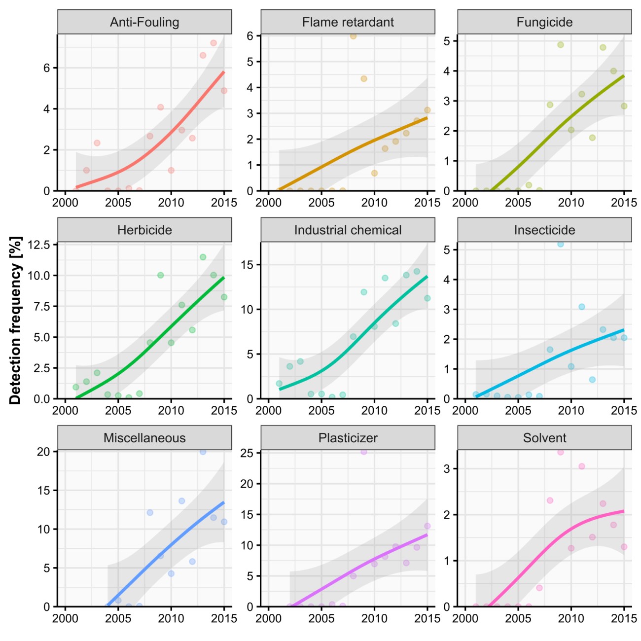
What can be found In European surface waters? Unfortunately, lots! What we found was rather alarming: all major chemical classes (e.g., pesticides, industrial chemicals, anti-fouling agents) were increasingly detected over time! This suggests that aquatic environments are more and more regularly exposed to these contaminants (Figure 3). For instance, in the most recent data (2012 – 2015), herbicides were detected in 10% of samples on average, and industrial chemicals are detected even more frequently. Pharmaceuticals were detected in ~ 50% of samples – that’s every second sample (data not shown in Figure 3).
We checked if analytical improvements or stochastic effects could potentially be the reason behind these increasing detection trends, but we found no evidence for that. Importantly, all of these substances don’t always occur alone, on the contrary, in most cases several of these contaminants would co-occur, which can further stress environments. You may also see that some chemical classes are rarely found, such as insecticides, solvents and even fungicides. While this may suggest a more environmentally benign character, this is most definitely not the case, as you will see in part 2 of this series.
Given these frequent detections, only around 30% of sites did not reveal any detectable organic contaminant in a given year. Taking a closer look at these sites, we found that the reason for non-detections wasn’t primarily because of their remote or pristine surroundings, but rather due to the employed monitoring methods being substantially flawed. The sampling frequency (i.e., how often water samples were taken) and the number of analyzed substances were both significantly lower (~ 40–50%) at these sites compared to sites where contaminants were found. We know that low sampling frequency and limited screening scope can substantially reduce the chance of capturing relevant toxicants. Therefore, it is likely that many of these sites did in fact contain organic contaminants, but they weren’t found due to suboptimal monitoring. The true environmental risk could therefore be higher than what we will talk about in Part 2 of this blogpost series.
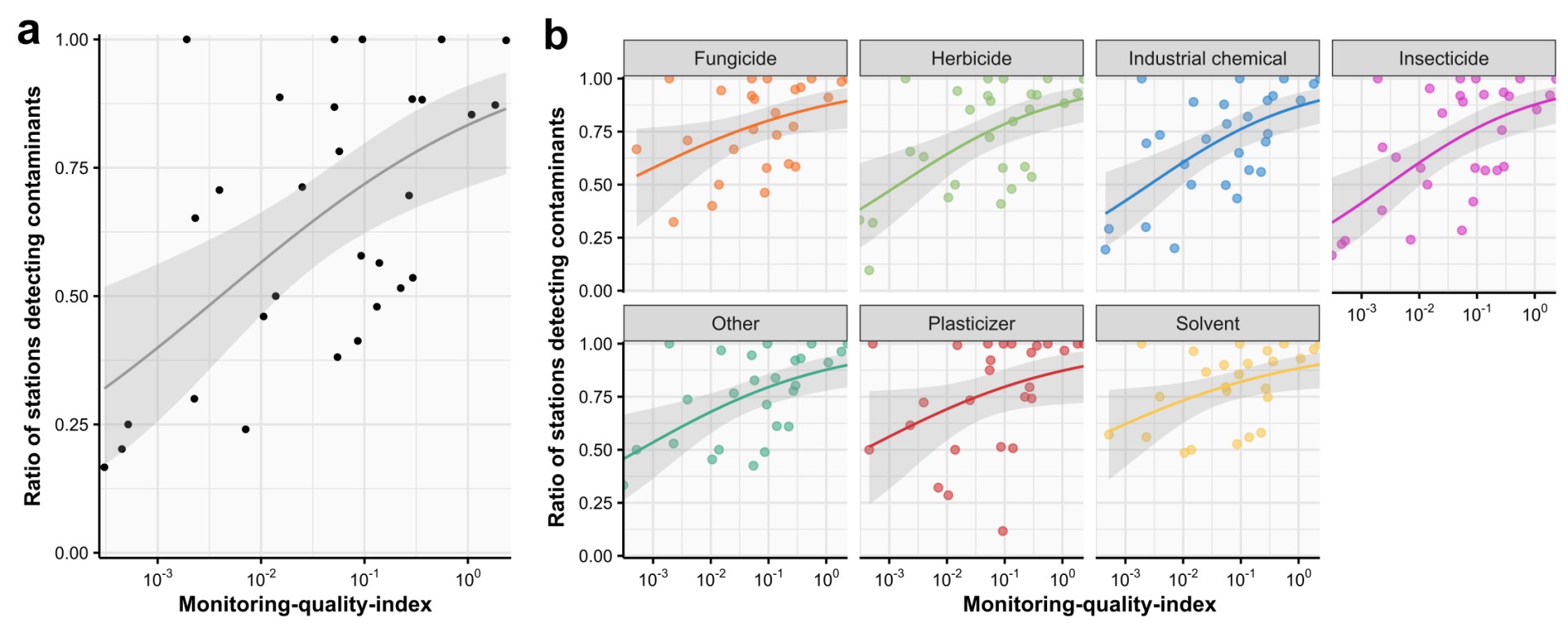
Keeping in mind that monitoring quality did differ considerably between countries and even between sites, we further investigated how monitoring quality (i.e., MQI) could impact the ability of detecting relevant contaminants in surface waters. It became clear that the MQI was correlated to these countries’ abilities of detecting toxic chemicals (Figure 4a): countries with a low MQI achieved far fewer detections spatially than those with a higher MQI (i.e., employing better monitoring strategies). This effect was also consistent across individual chemical classes (e.g., herbicides, industrial chemicals, Figure 4b), showing that our MQI serves as a crude but effective indicator.
Large data – big impact
These exercises confirmed that uncovering limitations of such large data troves is a key step for ecotoxicological evaluations on macro scales that needs to be undertaken prior to any other ecotoxicological analysis. We invested much time in these analyses, and wanted to take you along to help you tackling your next large data treasure. Identifying central data quality metrics and understanding their interactions will ultimately improve our perception of environmental risks and highlight the steps necessary to improve environmental monitoring.
With this first part of the blogpost series at hand, you should now have a better understanding which chemical classes occur in European surface waters, how important the quality of monitoring is, and that understanding large datasets is both necessary and rewarding for ecotoxicological assessments on macro scales.
This work was done as part of the research team “Meta-analysis of Global Impacts of Chemicals” (MAGIC) and if you are interested in our work, you can get in touch.
The paper was published by Jakob Wolfram, Sebastian Stehle, Sascha Bub, Lara Petschick, and Ralf Schulz in Environment International. Additionally, some interactive analyses (chemical association networks and Sankey-diagrams) can be accessed online here. Figures are reprinted with permission from Elsevier 2021 (CC-BY licence).