In this post, I provide an easy-to-use function to calculate confidence intervals in R.
One of the most handiest ways to present the precision of data is providing confidence intervals (CIs) as they are, amongst other reasons, readily interpretable and linked to statistical significance tests most (future) scientists are familiar with (Cumming & Finch 2001). However, in R receiving CIs can be quite cumbersome: either you calculate them on your own, perform hypothesis tests and extract the CIs from the respective output or use packages.
Some time ago, I thus wrote a function that allows to calculate CIs for means, medians, proportions as well as the differences of these for user-defined confidence levels according to the procedures described by Altman et al. (2000).
You can download the function as a txt file here.
To use the function, simply execute the whole provided code in your R console. The function uses the input parameters:
- x – your first or only sample
- y – your second sample in case you want to calculate a CI for a difference
- z – the confidence level expressed as a fraction, i.e., 0.95 for 95%
- type – either means, medians or proportions
- paired – this is only relevant if you want to calculate a CI for a mean or a median difference and the samples are paired
- k – the number of comparisons, in case you want to correct for multiple comparisons (the level of confidence is then adapted just as you might know it from a Bonferroni adjustment)
- na.rm – if you have missing data in your sample (i.e., NA) set this parameter to TRUE and it will be removed; otherwise missing data will prevent the function from working
Sounds rather complicated but in the end it’s quite easy. Let’s try a 95% CI for a mean of a sample with the values 3, 4, 5, 6:
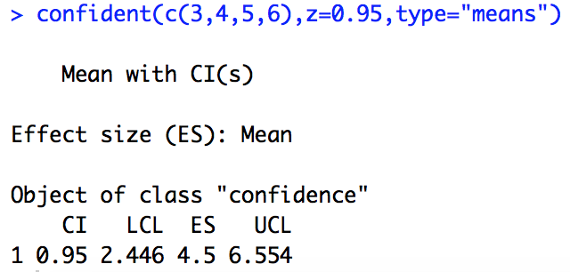
You receive an LCL (lower confidence level), an ES (effect size, in our case the mean), and a UCL (upper confidence level), which you all can access from the output object by using the $-symbol, for instance for use in plotting functions (e.g., plotCI from the plotrix package).
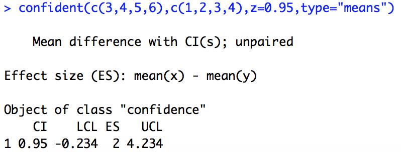
For a CI for the mean difference between two samples, we just additionally define the second sample y:
For proportions x and y (if used) need to be defined in a slightly different way as vectors each containing two numbers. The first is the number of observations with the specific feature you assess and the second number is your sample size. For instance, if 20 out of your 100 animals died during an experiment, you would write the following:
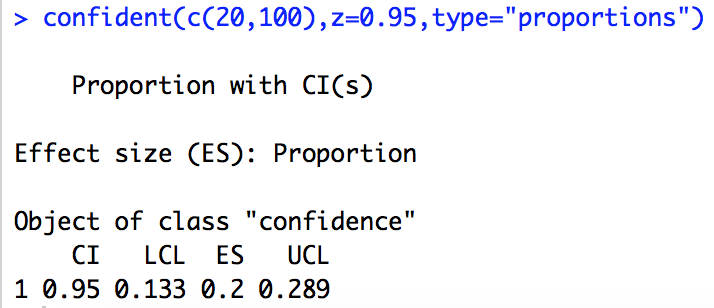
Note that your results are expressed as proportions now. So 0.2 means 20% of your animals are dead.
You see: no rocket science at all 🙂 Test the function and if you find any mistakes or have any questions, just let me know.
Cheers, Jochen
References used:
Altman DG, Machin D, Bryant TN, Gardner MJ eds. 2000. Statistics with confidence: confidence intervals and statistical guidelines, 2nd ed. BMJ books, London, UK.
Cumming G, Finch S. 2001. A Primer on the Understanding, Use, and Calculation of Confidence Intervals that are Based on Central and Noncentral Distributions. Educational and Psychological Measurement 61:532-574.